[논문 리뷰] Learning Pixel-level Semantic Affinity with Image-level Supervision for Weakly Supervised Semantic Segmentation

Abstract

• WSSS에서 local discriminative part는 잘 segment 하지만, entire object area에 대해서는 잘하지 못한다.
• AffinityNet은 local response를 nearby area로 propagate 시켜서 semantic entity를 얻는다.
• AffinityNet은 이러한 인접한 image coordinate pair 사이의 semantic affinity를 예측한다.
• 이러한 semantic propagation은 AffinityNet으로 부터 예측된 random walk로 구현된다.
• AffinityNet은 image-level class label만 필요로 하고, 그 외의 다른 데이터나 annotation은 필요로 하지 않는다.

Introduction

• Image-level의 WSSS에서는 추가적인 evidence를 이용해서 segmentation을 수행하는데, 이는 주로 CAM(Class Activation Map)을 이용한다.
• CAM을 통해 local discriminative part를 찾아내고, 이를 seed로 삼아서, entire object area로 propagate 시키는 방식을 사용한다.
• 이러한 방식에는 주로 image segmentation, motions in video를 이용하는 방식이 있다.
• 하지만, 이러한 방식은 extra data, off-the-shelf technique들이 필요하므로, 본 논문에서는 이러한 추가적인 data들이 필요없는 framework를 구성했다.

AffinityNet

• image를 input으로 받아서 인접한 image coordinate 사이의 semantic affinity를 예측하는 Network이다.
• process2) neighborhood graph를 구성하여 semantic affinity를 예측한다.
• 3) CAM은 neighborhood graph에 의해 random walk로 확장된다.
• 1) image와 그것의 CAM을 받아온다.

Contribution

• Image-level class label만으로, high-level semantic affinity를 예측하는 framework를 구성
• 다른 WSSS method와 달리, off-the-shelf technique에 의존하지 않음
• Image-level WSSS에서 SOTA를 달성했으며, FSSS 모델인 FCN보다 좋은 성능을 보임

Framework

• 전체적인 framework는 세가지 part로 구성되어 있다.
  • CAM
  • AffinityNet
  • DNN
  • ⇒ 앞의 CAM, AffinityNet은 segmentation label을 생성하는 part이며, DNN은 생성된 segmentation label로 segmentation을 수행하는 part이다.

Computing CAMs

• CAM은 WSSS에서 seed가 되는 부분으로, object의 local salient part를 찾아낸 후, propagate하며, entire object area를 찾아낸다.
• Architecture는 typical classification network에 GAP가 붙은 형태로 구성되어 있다.
  • GAP(Global Average Pooling)
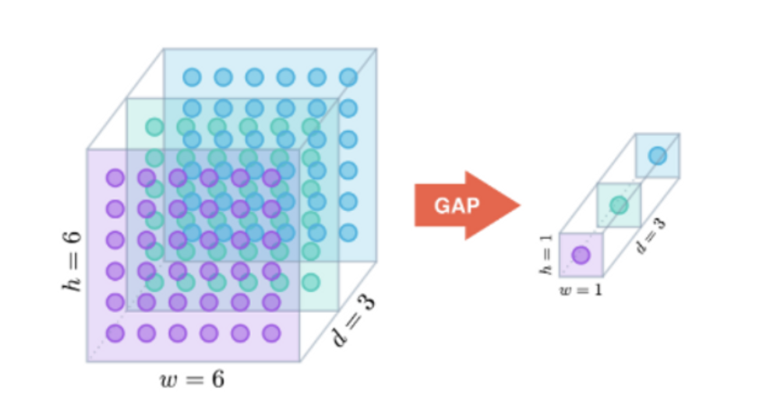
    • 각 feature map안에 있는 평균 값들을 output으로 출력하는 방식이다.
      
  $$
  M_c(x, y) = \mathbf{w}_c^\top f^{cam}(x, y)
  $$
  • $\mathbf{w}_c$ : classification weights
  • $f^{cam}(x, y)$ : feature vector located (x, y) on the feature map before GAP
  • $M_{bg}(x,y) = {1 - \max_{c \in C}M_c(x,y)}^\alpha$
• $$
  M_c(x,y) \rightarrow M_c(x,y) / \max_{x,y}M_c(x,y)
  $$

Learning AffinityNet

• AffininityNet은 random walk에 사용되는 affinity를 예측한다.
• 이는 CAM의 결과를 propagate하며, CAM의 퀄리티를 높인다.
• Computational efficiency를 위해 feature map의 인접한 coordinate 사이의 L1 Loss를 이용한다.
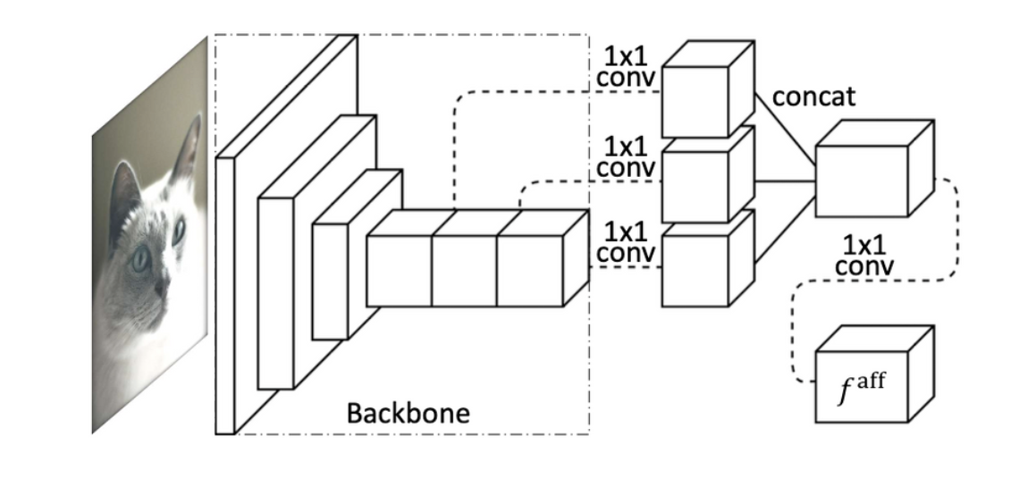
  • 여기서 $f^{aff}$는 아래의 architecture에 의해 생성되는데, 이 architecture를 training 시키는데에는 semantic affinity label이 필요하다.
  • 
• $$
  W_{ij} = \exp {-||f^{aff}(x_i, y_i) - f^{aff}(x_j, y_j)||_1}
  $$

Generating Semantic Affinity Labels

• CAM을 이용해서 object와 background의 confident area를 얻는 것이 기본적인 아이디어이다.
• Object의 confident area를 얻기 위해 다음과 같은 과정을 거친다.2) dCRF를 CAM에 적용시킨 후에 특정 class가 다른 class보다 score값이 높다면 특정 class에 대한 confident area로 생각할 수 있다.4) 그 외에 남은 영역은 중립 영역이라고 생각한다.
• 3) 동일한 방법으로 $\alpha$를 증가시켜 $M_{bg}$를 감소시켜서 confident background area를 찾아낼 수 있다.
• 1) $\alpha$를 감소시켜서 $M_{bg}$를 증폭시킨다. 그래서, background score가 다른 object의 activation score보다 두드러지게 한다.
• 이러한 과정을 거친 후에 인접한 픽셀간의 binary affinity를 측정하기 위해 두 위치가 모두 중립이 아니고, 같은 label이라면 $W_{ij}^* = 1$, 다른 label이면 $W_{ij}^* = 0$ 이라고 둔다.
  • 두 위치가 모두 중립이 아니면 무시한다.

AffinityNet Training

• AffinityNet은 binary affinity와 semantic affinity를 이용해서 gradient descent 방법으로 학습한다.
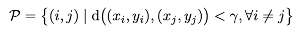
• Affinity는 다음과 같은 이유로 근접한 위치의 픽셀들 끼리의 관계만 고려해야한다.
  • 멀리 떨어져있는 픽셀간의 semantic affinity는 context가 부족하기 때문에 예측하기 힘들기 때문
  • computational cost를 낮출 수 있기 때문
• 그래서 set of coordinate pair를 다음과 같이 정의할 수 있다.
• 
• 하지만 이렇게 인접한 픽셀들에 대해 모두 training을 하면 class간에 밸런스가 맞지 않는 현상이 나타난다.$$
  \mathcal{P}^+ = \{(i,j)|(i,j) \in \mathcal{P}, W_{ij}^* = 1 \}
  $$
  • 최종적인 AffinityNet의 loss는 다음과 같다.
    $$
    \mathcal{L}{fg}^+ = - {1 \over | \mathcal{P}{fg}^+ |} \sum_{(i,j) \in \mathcal{P}{fg}^+} \log W{ij} \ \mathcal{L}{bg}^+ = - {1 \over | \mathcal{P}{bg}^+ |} \sum_{(i,j) \in \mathcal{P}{bg}^+} \log W{ij} \ \mathcal{L}^- = - {1 \over | \mathcal{P}^-|} \sum_{(i,j) \in \mathcal{P}^-} \log(1 - W_{ij}) \ \mathcal{L} = \mathcal{L}{fg}^+ + \mathcal{L}{bg}^+ + 2\mathcal{L}^-
    $$
  • 하지만 이렇게 구해진 loss는 class를 구분하지는 않는다.
  • ⇒ general representation을 학습하도록 한다.
    $$
    \mathcal{P}^- = \{(i,j)|(i,j) \in \mathcal{P}, W_{ij}^* = 0 \}
    $$
• 그래서 $\mathcal{P}$를 3 set으로 나누어, 각 subset에 대한 loss를 합치도록 하였다.

Revising CAMs Using AffinityNet

• AffinityNet에 의해 예측된 local semantic affinity는 transition probability matrix로 바뀐다.
• 이러한 transition matrix로 찾아낸 random walk는 CAM의 퀄리티를 향상시킨다.
• Transition matrix $T$는 다음과 같은 식으로 도출된다.
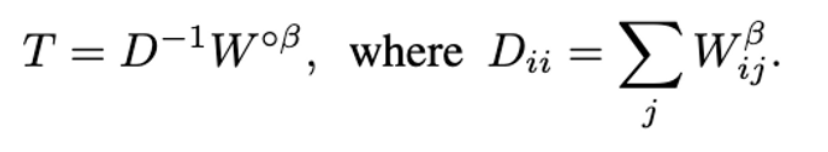
• 여기서 $W^{\circ \beta}$는 hadamard power를 의미하고, $\beta$는 1보다 큰 parameter로 중요하지 않은 affinity 값들을 무시하도록 해준다.
• 위 transition matrix로 semantic propagation을 수행한다.
  • t : number of iterations
• $vec(M_c^*) = T^t \cdot vec(M_c)$

Learning a Semantic Segmentation Network

• 향상된 CAM을 통해 segmentation label을 생성한다.
• 생성된 CAM은 원래 이미지보다 해상도가 낮기 때문에 bilinear interpolation을 통해 upsampling하고, dCRF를 통해 정교화한다.
• 이렇게 생성된 이미지와 label을 통해 semantic segmentation을 학습한다.

Netwokr Architecture

Backbone Network

• ResNet38을 수정하여 fully connected layer를 제거하고 마지막 3개 layer를 atrous convolution으로 교체하였다.
• Convolution dilation은 feature map이 stride 8을 가지도록 수행하였다.

Details of DNNs in Framework

• Network computing CAMs
  • backbone에 3x3x512 convolution layer, GAP, FC를 차례로 붙였다.
• AffinityNet
  • Backbone의 마지막 3개 layer의 출력을 선택하여 1x1 convolution을 이용해 차원을 128, 256, 512로 줄인 후에 이어붙였다.
  • 그 후 896 채널을 가지게 되었고, 여기에 1x1 convolution을 한번 더 이어 붙였다.
• Segmentation model
  • Backbone에 2개의 atrous convolution layer를 이어붙였고, 두 layer 모두 12의 dilation rate을 가진다.